IPL Exploratory Data Analysis

EDA on all IPL matches of seasons from 2008 to 2018. EDA is done using python, numpy, pandas, matplotlib, and seaborn.

IPL (Indian Premier League) is the most-attended cricket league in the world and in 2014 ranked sixth by average attendance among all sports leagues.

To enhance the capabilities of players, to decide on team composition and strategies, franchises may need concrete and precise analysis over the past plays & performance stats of the player and the team.

Getting a deeper understanding of the data is not possible using traditional methods.

Mumbai Indians franchise owners need to know all these stats to improve their chances of winning in the upcoming IPL seasons.

So for this analysis, Mumbai Indians is the team we will be doing analysis for and Wankhede Stadium is the home ground.

Please write to me if you need the source code of this EDA.

So let's get started with the EDA on IPL Dataset….

Installing & Importing Libraries

Installing Libraries

!pip install -q datascience                                         
!pip install -q pandas-profiling

Upgrading Libraries

• After upgrading the libraries, you need to restart the runtime to make the libraries in sync.
• Make sure not to execute the cell under Installing Libraries and Upgrading Libraries again after restarting the runtime.

!pip install -q --upgrade pandas-profiling

Importing Libraries

import pandas as pd
import numpy as np
from scipy import stats
import matplotlib.pyplot as plt
%matplotlib inline
import seaborn as sns
sns.set(style='whitegrid', font_scale=1.3, color_codes=True)
import warnings
warnings.filterwarnings('ignore')

Data Acquisition & Description

We will use below 2 datasets

1. Matches https://raw.githubusercontent.com/ravijagtap/datascience/main/IPL_DATA_ANALYSIS/datasets/matches.csv

This dataset contains details related to the match such as location, contesting teams, umpires, results, etc

2. Deliveries — https://raw.githubusercontent.com/ravijagtap/datascience/main/IPL_DATA_ANALYSIS/datasets/deliveries.csv

This dataset is the ball-by-ball data of all the IPL matches including data of the batting team, batsman, bowler, non-striker, runs scored, etc

Read Data from CSV

matches = pd.read_csv("https://raw.githubusercontent.com/insaid2018/Term-1/master/Data/Projects/matches.csv")
deliveries = pd.read_csv("https://raw.githubusercontent.com/insaid2018/Term-1/master/Data/Projects/deliveries.csv")

Data Profiling

Pandas have an open-source module ‘pandas_profiling’ using which we can quickly do EDA using just a few lines of code It generates interactive profile reports from a pandas DataFrame. The pandas df.describe() function is great but a little basic for serious EDA. pandas_profiling extends the pandas DataFrame with df.profile_report() for quick data analysis.

It can be installed using the below command if not already installed.

!pip install pandas_profiling==1.4.1
# import the required library
import pandas_profiling

Data profiling matches dataset.

# matches dataset profiling
matches_profile = matches.profile_report(title=”IPL Data Profiling before Data Processing of matches DF”, progress_bar=False, minimal=True)
matches_profile.to_file(output_file=”matches_profiling_before_processing.html”)

same for the deliveries dataset.

# deliveries dataset profiling
deliveries_profile = deliveries.profile_report(title="IPL Data Profiling before Data processing of deliveries DF", progress_bar=False, minimal=True)
deliveries_profile.to_file(output_file="deliveries_profiling_before_processing.html")

The report can be downloaded from here

matches_profiling_before_processing.html

deliveries_profiling_before_processing.html

Observations from Pandas Profiling of ‘matches’ Data set before Data Processing

1. matches Data set

Dataset info:

• Number of variables: 18
• Number of observations: 696
• Missing cells: 651 (5.2%)
• Duplicate Rows: 0

Variables types:

• Numeric = 4
• Categorical = 13
• Boolean = 1
• There are overall 11 seasons data in the data set.
• umpire3 has 636 (91.4%) missing values.
• city has 7 (1.0%) missing values.
• player_of_match has high cardinality of 214 distinct values.
• CH Gayle has got more player_of_match (20 times).
• out of 696 matches, we have got results for 686 matches, 7 were tie matches and 3 matches have no results.
• there were overall 19 matches where Duckworth lewis method was applied.

2. deliveries Data set

Dataset info:

• Number of variables: 21
• Number of observations: 1,64,750
• Missing cells: 472018 (13.6%)
• Duplicate Rows: 5

Variables types:

• Numeric = 10
• Categorical = 10
• Boolean = 1
• player_dismissed and dismissal_kind have 156593 missing values.
• batsman has high cardinality 488 distinct values.
• innings has values as 3 and 4, which means there were some matches in which super over was bowled.

Data Preprocessing

Get the dimensions of the datasets

— matches

matches.shape
(696, 18)

• There are 696 rows and 18 columns in the matches dataset

View the different data types in datasets

matches.info()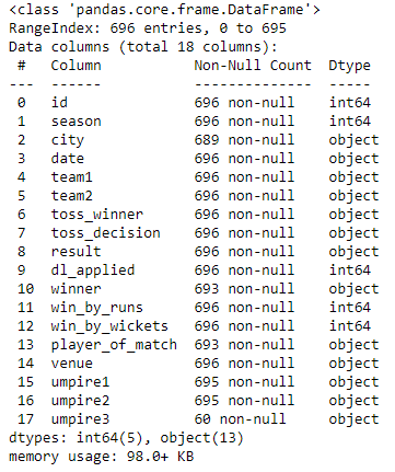

Check first 5 rows of matches dataset

matches.head()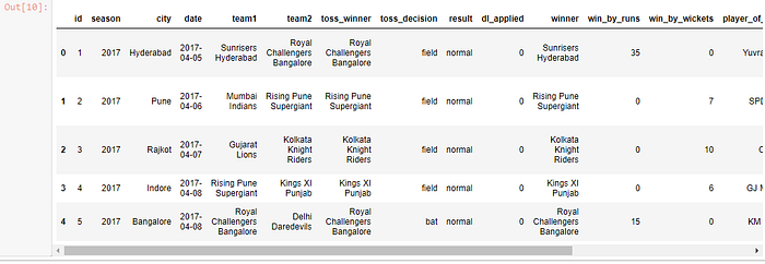

• Since the date is not relevant and does not provide any additional insights for our analysis, we will drop this column.
• umpire1, umpire2, and umpire3 can also be dropped for same reason.

matches.drop([‘date’, ‘umpire1’, ‘umpire2’, ‘umpire3’], axis=1, inplace=True)
# set id as the index column
matches.set_index('id', inplace=True)

— deliveries

deliveries.shape
(164750, 21)

There are 1,64,750 rows and 21 columns in the deliveries dataset

View the different data types in datasets

deliveries.info()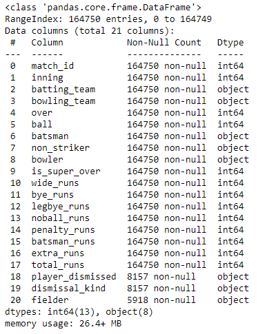

# set match_id as the index column
deliveries.set_index(‘match_id’, inplace=True)

Data Cleaning

Replacing the Full names with short names for ease of access

— matches dataset

#Replacing the Full names by short names
matches.replace(['Mumbai Indians','Kolkata Knight Riders','Royal Challengers Bangalore','Deccan Chargers','Chennai Super Kings',
                 'Rajasthan Royals','Delhi Daredevils','Gujarat Lions','Kings XI Punjab',
                 'Sunrisers Hyderabad','Rising Pune Supergiants','Kochi Tuskers Kerala','Pune Warriors','Rising Pune Supergiant']
                ,['MI','KKR','RCB','DC','CSK','RR','DD','GL','KXIP','SRH','RPS','KTK','PW','RPS'],inplace=True)

— deliveries dataset

#Replacing the Full names by short names
deliveries.replace(['Mumbai Indians','Kolkata Knight Riders','Royal Challengers Bangalore','Deccan Chargers','Chennai Super Kings',
                 'Rajasthan Royals','Delhi Daredevils','Gujarat Lions','Kings XI Punjab',
                 'Sunrisers Hyderabad','Rising Pune Supergiants','Kochi Tuskers Kerala','Pune Warriors','Rising Pune Supergiant']
                ,['MI','KKR','RCB','DC','CSK','RR','DD','GL','KXIP','SRH','RPS','KTK','PW','RPS'],inplace=True)

Rising Pune Supergiant is 2 times in the dataset one with the name Rising Pune Supergiant and the other as Rising Pune Supergiants, we replaced both with RPS

# merge seasons column in deliveries dataset which will be helpful in further analysis for each season
deliveries_seasons = deliveries.merge(matches["season"], left_on=deliveries.index, right_on=matches.index)

Exploratory Data Analysis

Exploratory Data Analysis(EDA) is an approach to analyzing data sets to summarize their main characteristics, often with visual methods.

• It includes cleaning, munging, combining, reshaping, slicing, dicing, and transforming data for analysis purposes.
• The primary goal of EDA is to maximize the analyst’s insight into a data set and into the underlying structure of a data set while providing all of the specific items that an analyst would want to extract from a data set.

Generic Stats

Q. How many seasons we’ve got in the dataset?

matches[‘season’].nunique()

print the season names

matches[‘season’].unique()

• we have got 11 seasons in the dataset from 2008 to 2018.

Q. How many matches were played in each season

seasons = matches['season'].value_counts().to_frame()
seasons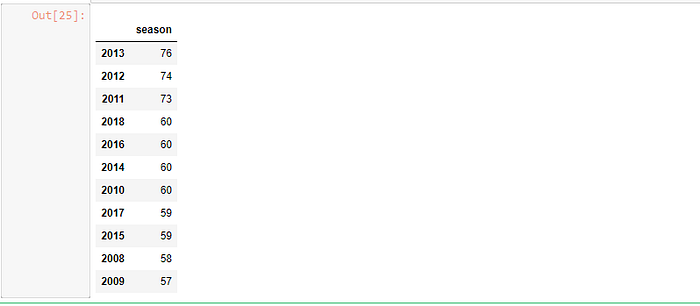

• This shows that most numbers of matches were played in the year 2013 (76 matches)

Plot this in a graph

seasons.plot(kind="bar", title="Number of matches per IPL seasons", figsize=(12,8))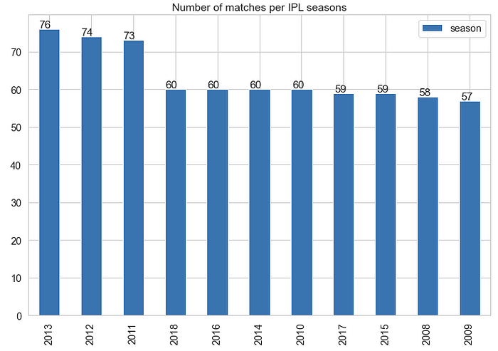

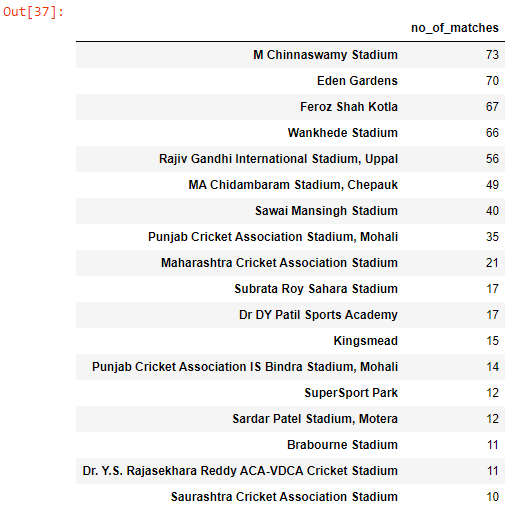
Q. How many matches were played in each venue?

no_of_matches = matches[‘venue’].value_counts().to_frame()
no_of_matches.rename(columns={‘venue’: ‘no_of_matches’}, inplace=True)
no_of_matches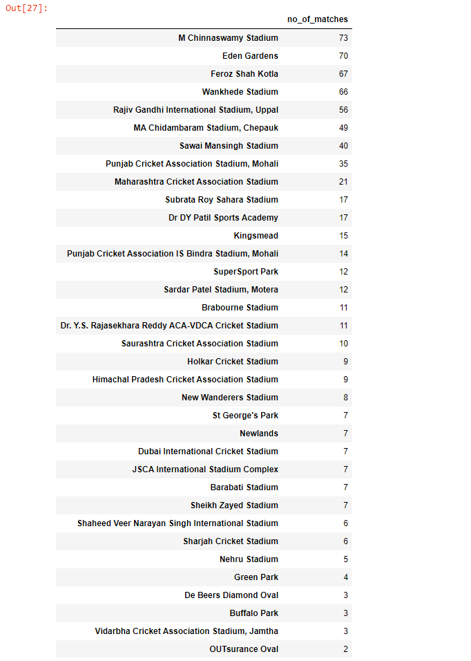

• M Chinnaswamy Stadium has hosted most matches (73).
• Wankhede Stadium is the 4th on the list and hosted 66 matches.
• There were some matches played outside India as well, like in cities Kingsmead, St George’s Park, etc.

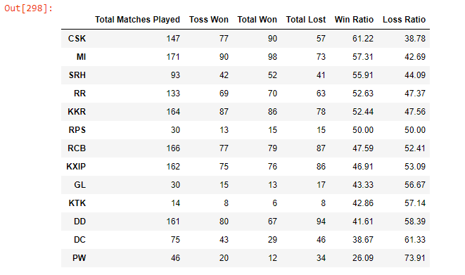
Q. Overview of matches played, toss won, wins, and losses for each team in the IPL history.

overall_team_stats = pd.DataFrame(
{‘Total Matches Played’: matches[“team1”].value_counts() +     matches[“team2”].value_counts(), 
‘Toss Won’: matches[“toss_winner”].value_counts(), ‘Total Won’: matches[“winner”].value_counts(), 
 ‘Total Lost’: ((matches[“team1”].value_counts() + matches[“team2”].value_counts()) — matches[“winner”].value_counts())})
overall_team_stats.sort_values(by=”Total Won”, ascending=False)

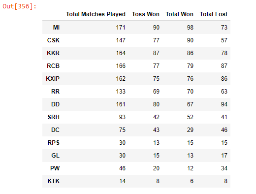
• Mumbai Indians has won most of the matches till now (98 times)

ax = overall_team_stats["Toss Won"].sort_values().plot(kind="barh", title="Number of Toss win in IPL", figsize=(12,8))
for p in ax.patches:
    ax.annotate(str(p.get_width()), (p.get_width() * 1.020, p.get_y() * 1.005))

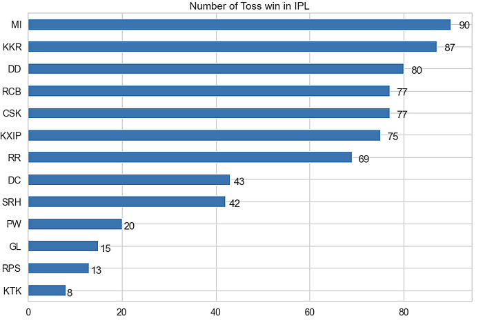
• MI has won most tosses till now i.e. 90 times

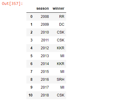
Q. List the winner of each season

season_winner = matches.drop_duplicates(subset=[‘season’], keep=’last’)[[‘season’, ‘winner’]]
season_winner.sort_values(by=”season”).reset_index(drop=True)

Q. Check the overall Win ratio of each team

overall_team_stats[‘Win Ratio’] = overall_team_stats[‘Total Won’] * 100 / overall_team_stats[‘Total Matches Played’]
overall_team_stats[‘Loss Ratio’] = overall_team_stats[‘Total Lost’] * 100 / overall_team_stats[‘Total Matches Played’]
overall_team_stats.round(2).sort_values(by=”Win Ratio”, ascending = False)

Q. Has Toss-winning helped in winning matches?

wins = matches[“toss_winner”] == matches[“winner”]
ax = wins.value_counts().plot(kind=”pie”, autopct=’%1.1f%%’, shadow=True)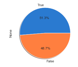

• This piechart shows that winning toss actually helped to win the match as well by 51.3%

Q. Check for each team what is the winning percentage when the team won the toss

# toss and match wins by toss_winner
toss_winner_as_winner = matches[matches[‘winner’] == matches[‘toss_winner’]].groupby([‘toss_winner’])[‘winner’].count()
# total toss wins by toss_winner
total_toss_winner = matches.groupby([‘toss_winner’])[‘winner’].count()
win_per_on_toss_win = toss_winner_as_winner / total_toss_winner * 100
win_per_on_toss_win = win_per_on_toss_win.to_frame()
win_per_on_toss_win[‘lost_per_on_toss_win’] = 100 — win_per_on_toss_win[‘winner’]
win_per_on_toss_win.rename(columns={‘winner’: ‘win_per_on_toss_win’}, inplace=True)
win_per_on_toss_win.round(2).sort_values(by=”win_per_on_toss_win”, ascending=False)

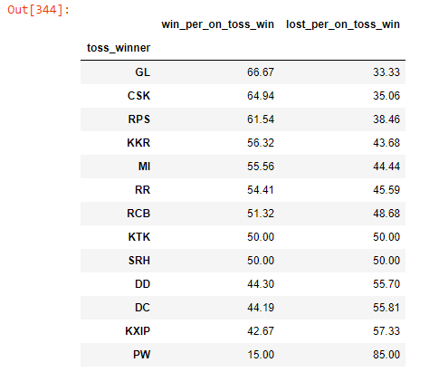
• Mumbai Indians won only 55.56% of the matches in which they won the toss

win_per_on_toss_win.plot.bar(figsize=(19,8), title=”Match Winning/Losing % of a team on winning the toss”,fontsize=13,
 cmap=’viridis’)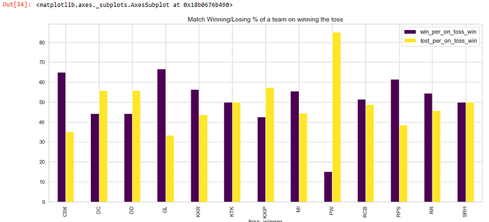

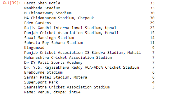
Q. Which stadium is best for winning by runs (most number of wins)?

stats.mode(matches[“venue”][matches[“win_by_runs”]!=0])

• Feroz Shah Kotla is the best stadium for winning by runs

Q. Which stadium is best for winning by wickets (most number of wins)?

stats.mode(matches[“venue”][matches[“win_by_wickets”]!=0])

• Eden Gardens is the best stadium for winning by wickets

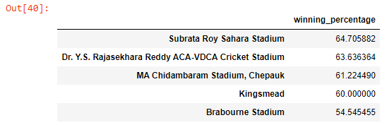
Q. Which are the top 5 stadiums for winning by runs against the number of matches played (at least 10 matches should have been played on the venue)?

atleast_10_mtch_at_venue = matches[‘venue’].value_counts().to_frame()
# Venues where atleast 10 matches are played
atleast_10_mtch_at_venue = atleast_10_mtch_at_venue[atleast_10_mtch_at_venue[‘venue’] >= 10][‘venue’].to_frame()
atleast_10_mtch_at_venue.rename(columns={‘venue’: ‘no_of_matches’}, inplace=True)
atleast_10_mtch_at_venue

# Filter the matches dataset to select on matches which were played in stadiums where atleast 10 matches were played
matches1 = matches[matches[‘venue’].isin(atleast_10_mtch_at_venue.index)]
matches1[matches1['win_by_runs'] > 0]['venue'].value_counts()

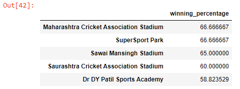
win_by_runs = matches1[matches1[‘win_by_runs’] > 0][‘venue’].value_counts() * 100 / matches1[‘venue’].value_counts() 
win_by_runs = win_by_runs.sort_values(ascending=False).head(5).to_frame()
win_by_runs.rename(columns={‘venue’: ‘winning_percentage’}, inplace=True)
win_by_runs

Q. Which are the top 5 stadiums for winning by wickets against the number of matches played (at least 10 matches should have been played on the venue)?

# Filter the matches dataset to select on matches which were played in stadiums where atleast 10 matches were played
matches2 = matches[matches[‘venue’].isin(atleast_10_mtch_at_venue.index)]
win_by_wickets = matches1[matches1['win_by_wickets'] > 0]['venue'].value_counts() * 100 / matches1['venue'].value_counts() 
win_by_wickets = win_by_wickets.sort_values(ascending=False).head(5).to_frame()
win_by_wickets.rename(columns={'venue': 'winning_percentage'}, inplace=True)
win_by_wickets

Q. Which is the best-chasing team?

matches[“winner”][matches[“win_by_wickets”]!=0].mode()

• Kolkata Knight Riders is the best team in chasing

Q. Does choosing batting or bowling first helped in match winning?

wins = matches[“toss_decision”][matches[“toss_winner”]==matches[“winner”]]
wins.value_counts().plot(kind=”pie”, autopct=’%1.1f%%’, shadow=True)

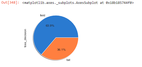
• From the above chart, we can say that choosing fielding first by toss winner helped in winning the match as well

Mumbai Indians Stats

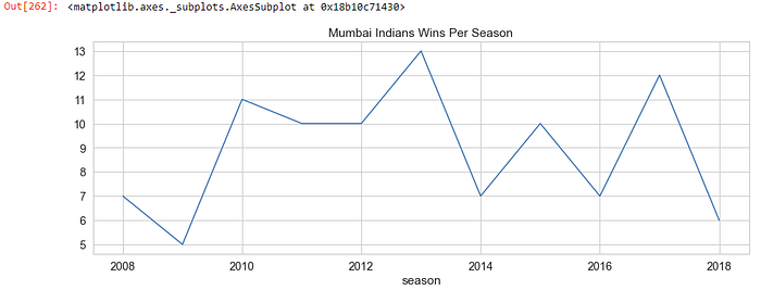
Q. The number of matches won by Mumbai Indians per season?

no_of_wins = matches[matches[‘winner’] == ‘MI’].groupby([‘season’]).count()
no_of_wins[“winner”].plot(kind=”line”, figsize=(15, 5), title=”Mumbai Indians Wins Per Season”)

Q. For MI which stadium is best when they win the toss?

matches[“venue”][matches[“toss_winner”]==”MI”][matches[“winner”]==”MI”].mode()

• Wankhede Stadium is the best when MI win the toss

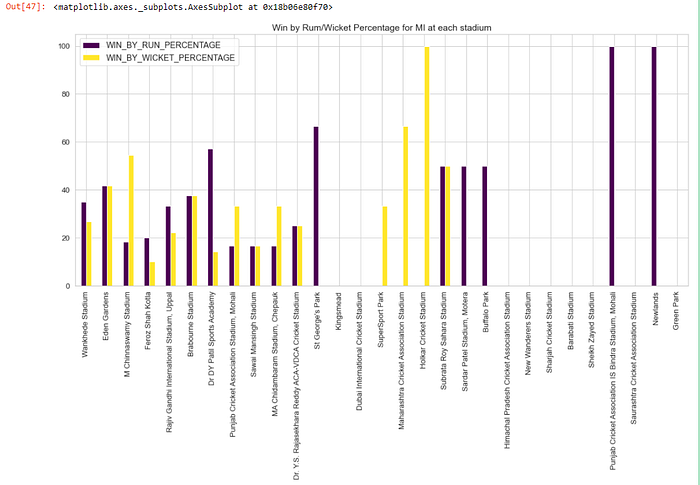
Q. Does batting first or bowling first helped in match winning for Mumbai Indians at each venue?

# filter matches which MI played
mi_matches = matches[(matches['team1'] == "MI") | (matches['team2'] == "MI")]
mi_total_matches = mi_matches["venue"].value_counts().to_frame()
mi_total_matches.rename(columns={'venue': 'NO_OF_MATCHES_AT_VENUE'}, inplace=True)
#filter where MI is winner and win is by Run
win_by_runs = mi_matches[(mi_matches['winner'] == "MI") & (mi_matches["win_by_runs"] > 0)]
win_by_runs_count = win_by_runs['venue'].value_counts().to_frame()
win_by_runs_count.rename(columns={'venue': 'MI_WINS_BY_RUNS'}, inplace=True)
#filter where MI is winner and win is by wickets
win_by_wickets = mi_matches[(mi_matches['winner'] == "MI") & (mi_matches["win_by_wickets"] > 0)]
win_by_wickets_count = win_by_wickets['venue'].value_counts().to_frame()
win_by_wickets_count.rename(columns={'venue': 'MI_WINS_BY_WICKETS'}, inplace=True)
# merge the datasets
frames = [mi_total_matches, win_by_runs_count, win_by_wickets_count]
result = pd.concat(frames, axis=1)
#get the percentage of totals wins over total matches played
result["MI_NO_OF_LOSS"] =  result["NO_OF_MATCHES_AT_VENUE"]  - result["MI_WINS_BY_RUNS"] - result["MI_WINS_BY_WICKETS"];
result["WIN_BY_RUN_PERCENTAGE"] = result["MI_WINS_BY_RUNS"] * 100 / result["NO_OF_MATCHES_AT_VENUE"]
result["WIN_BY_WICKET_PERCENTAGE"] = result["MI_WINS_BY_WICKETS"] * 100 / result["NO_OF_MATCHES_AT_VENUE"]
result[["WIN_BY_RUN_PERCENTAGE", "WIN_BY_WICKET_PERCENTAGE"]].plot.bar(figsize=(19,8), title="Win by Rum/Wicket Percentage for MI at each stadium",fontsize=13, cmap='viridis')

Q. Hows the performance of MI at home ground (Wankhade)

result.iloc[0, 1:4].plot(kind=’pie’, fontsize=14, autopct=’%3.1f%%’, title=”Win by Run/Wicket and Losses for MI at Wankhade”, 
 figsize=(10,10), shadow=True, startangle=135, legend=True, cmap=’summer’)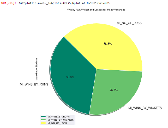

• Mumbai Indians played most matches at Wankhede Stadium where batting first helped them winning the match by 35%

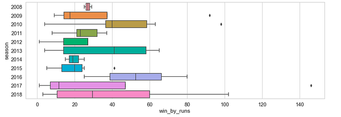
Q. MI Performance — Winning by Runs

#Winning by Runs — Team Performance
plt.figure(figsize=(15,5))
sns.boxplot(y = ‘season’, x = ‘win_by_runs’, data=matches[(matches[‘win_by_runs’] > 0) & (matches[“team1”] == “MI”)], orient = ‘h’);
plt.show()

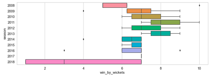
Q. MI Performance — Winning by Wickets

# Winning by Wickets — Team Performance
plt.figure(figsize=(15,5))
sns.boxplot(y = ‘season’, x = ‘win_by_wickets’, data=matches[(matches[‘win_by_wickets’] > 0) & (matches[“team1”] == “MI”)], orient = ‘h’);
plt.show()

Q. Against which team Mumbai Indians got the most defeats

mi_defeats = mi_matches[mi_matches[‘winner’] != “MI”][‘winner’].value_counts().to_frame()
mi_defeats.rename(columns={‘winner’: ‘number_of_defeats’}, inplace=True)
mi_defeats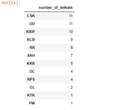

• CSK and DD defeated MI 11 times

Q. Check if CSK and DD opted to field or bat first in these matches in which MI got defeat

csk_dd = [“CSK”, “DD”]
mi_csk_dd_matches = mi_matches[(mi_matches[‘winner’] != “MI”) & (mi_matches[‘team1’].isin(csk_dd) | mi_matches[‘team2’].isin(csk_dd))]
mi_csk_dd_matches[‘opted_for’]=mi_csk_dd_matches[“win_by_runs”].apply(lambda x : “BAT” if(x > 0) else “FIELD”)
plt.figure(figsize=(15,5))
mi_csk_dd_matches[mi_csk_dd_matches[“opted_for”] == “FIELD”].groupby([“winner”])[“opted_for”].value_counts().plot(kind=’bar’, color=’blue’)
mi_csk_dd_matches[mi_csk_dd_matches[“opted_for”] == “BAT”].groupby([“winner”])[“opted_for”].value_counts().plot(kind=’bar’, color=’red’, fontsize=13)
plt.ylabel(“No_of_matches”)
plt.xticks([0, 1], [“CSK”, “DD”])
plt.legend([‘Field First’, ‘Bat First’])
plt.show()

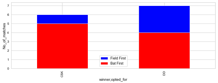
• Most of the times both CSK and DD opted to field first against MI in which MI lost the matches

Q. For MI which bowler gave the most extra runs (top 5 only) (take only bowlers who bowled atleast 24 deliveries). Find the % of extra over total balls bowled

no_of_deliveries_per_bowler = deliveries[deliveries[“bowling_team”] == “MI”].groupby(“bowler”)[“bowler”].count().to_frame()
no_of_deliveries_per_bowler.rename(columns={‘bowler’: ‘no_of_deliveries’}, inplace=True)
no_of_deliveries_per_bowler_atleast24 = no_of_deliveries_per_bowler[no_of_deliveries_per_bowler[“no_of_deliveries”] > 24]
total_extra_runs = deliveries[deliveries[“bowling_team”] == “MI”].groupby(“bowler”)[“extra_runs”].sum().to_frame()
total_extra_runs.rename(columns={‘extra_runs’: ‘no_of_deliveries’}, inplace=True)
perc = total_extra_runs * 100 / no_of_deliveries_per_bowler_atleast24
perc.sort_values(by=”no_of_deliveries”, ascending=False).head(5).plot(kind=”bar”, figsize=(15, 5), title=”% of extra runs over deliveries bowled”)

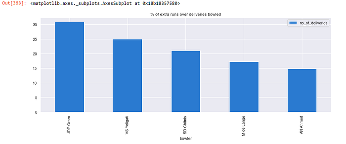
• JDP Oram gave the most runs in extra

Powerplay

Powerplay is of 6 overs for both innings of the match. During powerplay there is a field restriction. During this overs teams try to score maximum runs or try to take more wickets

Q. Compare total runs scored by each team throught IPL in power play

runs_per_team = deliveries_seasons[(deliveries_seasons[“over”] <= 6)].groupby(deliveries_seasons[“batting_team”])[“total_runs”].sum()
ax = runs_per_team.plot(kind=”bar”, figsize=(20,10), title=”Total Runs by Each Team in powerplay”)
for p in ax.patches:
 ax.annotate(str(p.get_height()), (p.get_x() * 1.005, p.get_height() * 1.005))

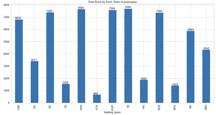
• MI scored the highest number of runs (7690) throughtout the IPL season in power plays

Q. Compare total wickets taken by each team throught IPL in power play

wick_in_powerplay_per_match_per_season = deliveries_seasons[(deliveries_seasons[“over”] <= 6) & (deliveries_seasons[“player_dismissed”].notnull())].groupby(deliveries_seasons[“bowling_team”])[“player_dismissed”].count()
ax = wick_in_powerplay_per_match_per_season.plot(kind=”bar”, figsize=(20,10), title=”Total Wickets by Each Team in powerplay”)
for p in ax.patches:
 ax.annotate(str(p.get_height()), (p.get_x() * 1.005, p.get_height() * 1.005))

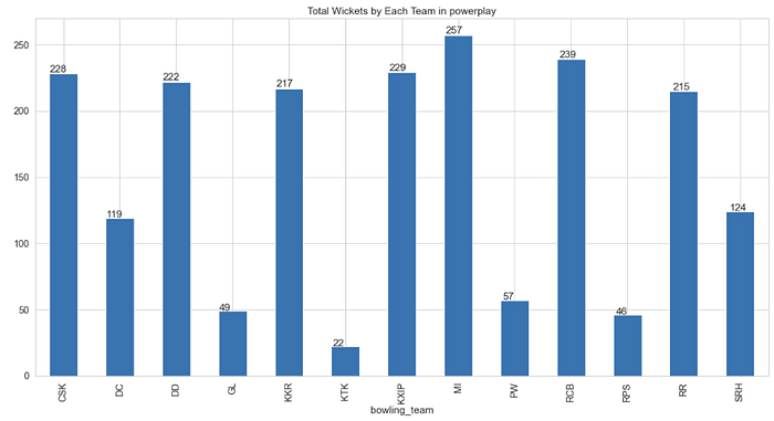
• MI took the highest number of wickets (257) in powerplays

Q. Which team scored highest runs in powerplay against MI

runs_per_team = deliveries_seasons[(deliveries_seasons[“over”] <= 6) & (deliveries_seasons[“bowling_team”] == “MI”)].groupby(deliveries_seasons[“batting_team”])[“total_runs”].sum()
ax = runs_per_team.plot(kind=”bar”, figsize=(20,10))
for p in ax.patches:
 ax.annotate(str(p.get_height()), (p.get_x() * 1.005, p.get_height() * 1.005))

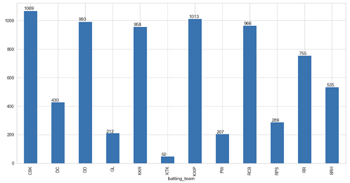
• CSK scored maximum runs in powerplay (1069) followed by KXIP (1013) in powerplay

Q. Which team took most MI wickets in powerplay

wick_in_powerplay_per_match_per_season = deliveries_seasons[(deliveries_seasons[“batting_team”] == “MI”) & (deliveries_seasons[“over”] <= 6) & (deliveries_seasons[“player_dismissed”].notnull())].groupby(deliveries_seasons[“bowling_team”])[“player_dismissed”].count()
ax = wick_in_powerplay_per_match_per_season.plot(kind=”bar”, figsize=(20,10), title=”Total Wickets by Each Team in powerplay”)
for p in ax.patches:
 ax.annotate(str(p.get_height()), (p.get_x() * 1.005, p.get_height() * 1.005))

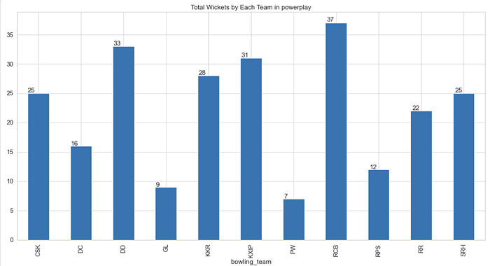
• RCB took most MI wickets (37) followed by DD (33) in powerplay

Further Breakdown of the runs and wickets in powerplay per season

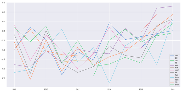
Q. Check average runs scored in powerplay by each team per season

teams = np.sort(matches[“team1”].unique())
plt.figure(figsize=(20,10))
for key, team in enumerate(teams): 
 run_in_powerplay_per_match_per_season = deliveries_seasons[(deliveries_seasons[“batting_team”] == team) & (deliveries_seasons[“over”] <= 6)].groupby([“key_0”, “season”])[“total_runs”].sum().to_frame() 
 a = run_in_powerplay_per_match_per_season.groupby([“season”])[“total_runs”].mean() 
 plt.plot(list(a.index), a, label = team)
 
plt.legend()
plt.show()

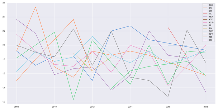
Q. Check average wickets taken by a team in powerplay by per season

teams = np.sort(matches[“team1”].unique())
plt.figure(figsize=(20,10))
for key, team in enumerate(teams): 
 wick_in_powerplay_per_match_per_season = deliveries_seasons[(deliveries_seasons[“bowling_team”] == team) & (deliveries_seasons[“over”] <= 6) & (deliveries_seasons[“player_dismissed”].notnull())].groupby([“key_0”, “season”])[“season”].count() 
 a = wick_in_powerplay_per_match_per_season.groupby([“season”]).mean() 
 plt.plot(list(a.index), a, label = team)
 
plt.legend()
plt.show()

Q. For MI which player has the maximum strike rate in powerplays

mi_batsman = deliveries_seasons[(deliveries_seasons[“batting_team”] == “MI”) & (deliveries_seasons[“over”] <= 6)]
batsman_mean = (mi_batsman.groupby(“batsman”)[“batsman_runs”].mean() * 100).round(2)
ax = batsman_mean.sort_values(ascending = False).head(5).plot(kind=”bar”, figsize=(15,5))
for p in ax.patches:
 ax.annotate(str(p.get_height()), (p.get_x() * 1.005, p.get_height() * 1.005))

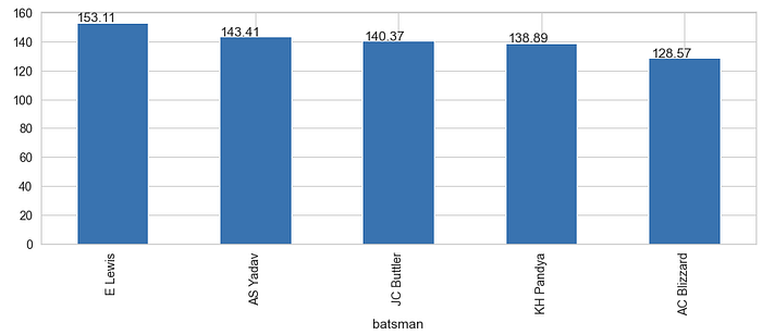
• E Lewis has the maximum strike rate of 166

Q. For MI which bowler is most economical in powerplays, the bowler must have bowled at least 20 overs overall

mi_bowlers = deliveries_seasons[(deliveries_seasons[“bowling_team”] == “MI”) & (deliveries_seasons[“over”] <= 6)]
total_runs = mi_bowlers.groupby(“bowler”)[“total_runs”].sum().to_frame()
overs_per_match = mi_bowlers[mi_bowlers[“ball”] <= 6].groupby([“key_0”, “bowler”])[“over”].nunique().to_frame()
total_overs = overs_per_match.groupby(“bowler”).sum()
# bowler bowled atleat 20 overs
total_overs = total_overs[total_overs[“over”] >= 20]
economic_rate = total_runs[“total_runs”] / total_overs[“over”]
economic_rate.sort_values(ascending = True).head(5)
ax = economic_rate.sort_values(ascending = True).round(2).head(5).plot(kind=”bar”, figsize=(15,5))
for p in ax.patches:
 ax.annotate(str(p.get_height()), (p.get_x() * 1.005, p.get_height() * 1.005))

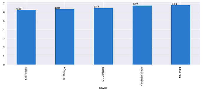
• SM Pollock is the most economical baller for MI

Q. Which bowler has taken most wickets against MI

mi_wickets = deliveries_seasons[(deliveries_seasons[“batting_team”] == “MI”) & (deliveries_seasons[“player_dismissed”].notnull())].groupby(deliveries_seasons[“bowler”])[“player_dismissed”].count()
ax = mi_wickets.sort_values(ascending = False).head(5).plot(kind=”bar”, figsize=(15,5))
for p in ax.patches:
 ax.annotate(str(p.get_height()), (p.get_x() * 1.005, p.get_height() * 1.005))

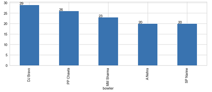
• DJ Bravo has taken the most wickets (29) against MI

Q. For MI which players partnership is successful

deliveries[deliveries[“batting_team”] == “MI”].groupby([“batsman”, “non_striker”])[“total_runs”].sum().sort_values(ascending = False).to_frame()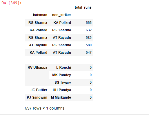

• RG Sharma and KA Pollards patnership is the most successful (666 + 632 = 1298 Runs) for MI followed by RG Sharma and AT Rayudu (585 + 580 = 1165 Runs)

Q. Which top 5 batsmen are most successful in super overs

super_overs = deliveries[deliveries[“is_super_over”] == 1].groupby(“batsman”)[“total_runs”].sum().sort_values(ascending = False).head()
super_overs.plot(kind=”bar”, figsize=(15, 5))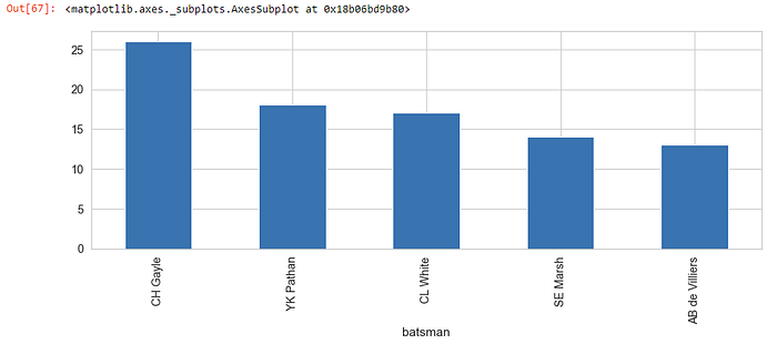

Q. Which top 5 bowlers are most successful in super overs in terms of wickets

super_overs = deliveries[(deliveries[“is_super_over”] == 1) & (deliveries[“player_dismissed”].notnull())].groupby(“bowler”)[“player_dismissed”].count().sort_values(ascending = False).head()
super_overs.plot(kind=”bar”, figsize=(15, 5))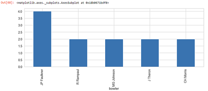

Awards

In IPL there are different awards that are being given to players. They are Orange Cap, Purple Cap, Maximum Sixes Award, Most Valuable Player and Emerging Player of the Year. Will find out which players got Orange Cap and Purple Cap awards per season

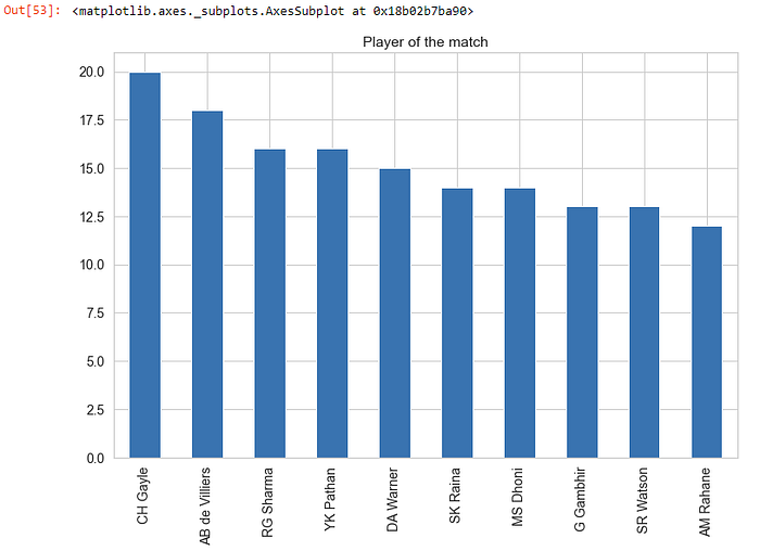
Q. Top player of the match Winners

top_players = matches[“player_of_match”].value_counts().head(10)
top_players.plot(kind=”bar”, title=”Player of the match”, figsize=(12,8))

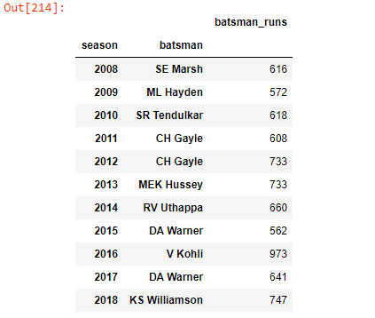
Q. Orange Cap Winner Per Season

The Orange Cap is presented to the leading run scorer in the season

orange_cap_players = deliveries_seasons.groupby([“season”]).apply(lambda x: (
 x.groupby([“batsman”]).sum()
 .sort_values(‘batsman_runs’, ascending=False)).head(1))
orange_cap_players[“batsman_runs”].to_frame()

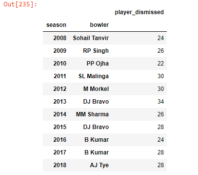
Q. Purple Cap Winner Per Season

The Purple Cap is presented to the leading wicket-taker in the season

orange_cap_players = deliveries_seasons[deliveries_seasons[“player_dismissed”].notnull()].groupby([“season”]).apply(lambda x: (
 x.groupby([“bowler”]).count()
 .sort_values(“player_dismissed”, ascending=False)).head(1))
orange_cap_players[“player_dismissed”].to_frame()

Q. Who is the most valuable player for MI (based on MOM)

mi_matches[mi_matches[“winner”] == “MI”][“player_of_match”].value_counts().head(1)

• Rohit Sharma is the most valuable player for MI

Q. Players with most 4s and 6s

deliveries[deliveries[“batsman_runs”] == 4].groupby(“batsman”)[“batsman_runs”].count().sort_values(ascending = False).head(10).plot(kind=’bar’, title=”Top 10 players with most 4s”, figsize=(15,7), color=’orange’)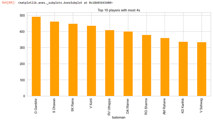

deliveries[deliveries[“batsman_runs”] == 6].groupby(“batsman”)[“batsman_runs”].count().sort_values(ascending = False).head(10).plot(kind=’bar’, title=”Top 10 Players with most 6s”, figsize=(15,7), color=’green’)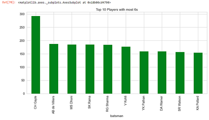

Conclusion

• We have got the dataset with data for 11 IPL seasons from 2008 to 2018
• Total matches played in these seasons is 696
• Most number of matches which is 76 were played in season 2013
• Most number of matches which is 73, were played in M Chinnaswamy Stadium
• Mumbai Indians played most matches which is 171 followed by RCB 166
• Mumbai Indians won most matches 98 followed by CSK 90
• Mumbai Indians and CSK have won 3 seasons each
• Mumbai Indians in 2013, 2015 and 2017
• CSK in 2010, 2011 and 2018
• CSK has the best winning percentage of 61.22% and Pune Warriors has worst winning percentage of 26.09%
• GL has has best winning percentage of 66.67 followed by CSK with 64.93% when they won the toss as well.
• Winning a team has actually helped the team to win the match as well by 51.3%
• Mumbai Indians won only 55.56% of the matches in which they won the toss
• Feroz Shah Kotla stadium is the best stadium for winning by runs
• Eden Gardens is the best stadium for winning by wickets
• Kolkata Knight Riders is good at defending the total
• 63.9% time a team has won the match if the team has won the toss as well and choose to field first
• Mumbai Indians won most matches in season 2013
• Wankhede Stadium is the best for MI to win the match when they also win the toss
• Mumbai Indians played most matches at Wankhede Stadium where batting first helped them winning the match by 35%
• CSK and DD defeated MI 11 times, where most of the times both CSK and DD opted to field first against MI
• For mumbai Indians “JDP Oram” gave the most runs in extra
• MI scored the highest number of runs (7690) throughtout the IPL season in power plays
• MI took the highest number of wickets (257) in powerplays
• CSK scored maximum runs in powerplay (1069) followed by KXIP (1013) in powerplay
• RCB took most MI wickets (37) followed by DD (33) in powerplay
• For Mumbai Indians, ‘E Lewis’ has the maximum strike rate of 166 during powerplay
• SM Pollock is the most economical baller with economy of 6.26 per over for MI during powerplay
• DJ Bravo has taken most wickets (29) against MI
• RG Sharma and KA Pollards patnership is the most successful (666 + 632 = 1298 Runs) for MI followed by RG Sharma and AT Rayudu (585 + 580 = 1165 Runs)
• Overall CH Gayle has scored most runs in a superover
• JP Faulkner has taken most wickets in superover
• CH Gayle has got most man of the match award i.e. 20 times
• Rohit Sharma is the most valuable player for MI
• G Gambhir has scored most 4s in IPL history
• CH Gayle has scored most 6s in IPL history